(Open Source Geospatial Python)

The ‘What is it?’

The Standard Distance, also know as the Standard Distance Deviation, is the average distance all features vary from the Mean Center and measures the compactness of a distribution. The Standard Distance is a value representing the distance in units from the Mean Center and is usually plotted on a map as a circle for a visual indication of dispersion, the Standard Distance is the radius.

The Standard Distance works best in the absence of a strong directional trend. According to Andy Mitchell, if a directional trend is present you are better off using the Standard Deviational Ellipse.

You can use the Standard Distance to compare territories between species, which has the wider/broader territory, or to compare changes over time such as the dispersion of burglaries for each calendar month.

In a Normal Distribution you would expect around 68% of all points to fall within the Standard Distance.

The Formula!

The mean x-coordinate is subtracted from the x-coordinate value for each point and the difference is squared. The sum of all the squared values for x minus the x-mean is divided by the number of points. This is also performed for y-coordinates. The resulting values for x and y are summed and then we take the square root of this value to return the value to original distance units.

First we get the mean X and Y…

…and then the Standard Distance

For Point features the X and Y coordinates of each feature is used, for Polygons the centroid of each feature represents the X and Y coordinate to use, and for Linear features the mid-point of each line is used for the X and Y coordinate.

The Code…

from osgeo import ogr
from shapely.geometry import MultiLineString
from shapely import wkt
import numpy as np
import sys, math

## set the driver for the data
driver = ogr.GetDriverByName("FileGDB")
## path to the FileGDB
gdb = r"C:\Users\Glen B\Documents\ArcGIS\Default.gdb"
## ope the GDB in write mode (1)
ds = driver.Open(gdb, 1)

input_lyr_name = "Birmingham_Burglaries_2016"

output_fc = "{0}_standard_distance".format(input_lyr_name)

## reference the layer using the layers name
if input_lyr_name in [ds.GetLayerByIndex(lyr_name).GetName() for lyr_name in range(ds.GetLayerCount())]:
    lyr = ds.GetLayerByName(input_lyr_name)
    print "{0} found in {1}".format(input_lyr_name, gdb)

if output_fc in [ds.GetLayerByIndex(lyr_name).GetName() for lyr_name in range(ds.GetLayerCount())]:
    ds.DeleteLayer(output_fc)
    print "Deleting: {0}".format(output_fc)

try:
    ## for points and polygons we use the centroid
    first_feat = lyr.GetFeature(1)
    if first_feat.geometry().GetGeometryName() in ["POINT", "MULTIPOINT", "POLYGON", "MULTIPOLYGON"]:
        xy_arr = np.ndarray((len(lyr), 2), dtype=np.float)
        for i, pt in enumerate(lyr):
            ft_geom = pt.geometry()
            xy_arr[i] = (ft_geom.Centroid().GetX(), ft_geom.Centroid().GetY())

    ## for lines we get the midpoint of a line
    elif first_feat.geometry().GetGeometryName() in ["LINESTRING", "MULTILINESTRING"]:
        xy_arr = np.ndarray((len(lyr), 2), dtype=np.float)
        for i, ln in enumerate(lyr):
            line_geom = ln.geometry().ExportToWkt()
            shapely_line = MultiLineString(wkt.loads(line_geom))
            midpoint = shapely_line.interpolate(shapely_line.length/2)
            xy_arr[i] = (midpoint.x, midpoint.y)

except Exception:
    print "Unknown geometry for {}".format(input_lyr_name)
    sys.exit()

avg_x, avg_y = np.mean(xy_arr, axis=0)

print "Mean Center: {0}, {1}".format(avg_x, avg_y)

sum_of_sq_diff_x = 0.0
sum_of_sq_diff_y = 0.0

for x, y in xy_arr:
    diff_x = math.pow(x - avg_x, 2)
    diff_y = math.pow(y - avg_y, 2)
    sum_of_sq_diff_x += diff_x
    sum_of_sq_diff_y += diff_y

sum_of_results = (sum_of_sq_diff_x/lyr.GetFeatureCount()) + (sum_of_sq_diff_y/lyr.GetFeatureCount())
standard_distance = math.sqrt(sum_of_results)
print "Standard Distance: {0}". format(standard_distance)

## create a point with the mean center
## and buffer by the standard distance
pnt = ogr.Geometry(ogr.wkbPoint)
pnt.AddPoint(avg_x, avg_y)
polygon = pnt.Buffer(standard_distance, 90)

## create a new polygon layer with the same spatial ref as lyr
out_lyr = ds.CreateLayer(output_fc, lyr.GetSpatialRef(), ogr.wkbPolygon)

## define and create new fields
x_fld = ogr.FieldDefn("X", ogr.OFTReal)
y_fld = ogr.FieldDefn("Y", ogr.OFTReal)
stnd_dst = ogr.FieldDefn("Standard_Distance", ogr.OFTReal)
out_lyr.CreateField(x_fld)
out_lyr.CreateField(y_fld)
out_lyr.CreateField(stnd_dst)

## add the standard distance buffer to the layer
feat_dfn = out_lyr.GetLayerDefn()
feat = ogr.Feature(feat_dfn)
feat.SetGeometry(polygon)
feat.SetField("X", avg_x)
feat.SetField("Y", avg_y)
feat.SetField("Standard_Distance", standard_distance)
out_lyr.CreateFeature(feat)

print "Created {0}".format(output_fc)

## free up resources
del feat, ds, lyr, out_lyr

I’d like to give credit to Logan Byers from GIS StackExchange who aided in speeding up the computational time using NumPy and for forcing me to begin learning the wonders of NumPy (getting there bit by bit).

The Example:

I downloaded crime data from DATA.POLICE.UK for the West Midlands Police from January 2016 to December 2016. I used some Python to extract just the Burglary data and made this into a feature class in the File GDB. Next, I downloaded OS Boundary Line data and clipped the Burglary data to just Birmingham. Everything was now in place to find the Standard Distance of all burglaries for Birmingham in 2016. (see The Other Scripts section at the bottom of this post for processing the data)

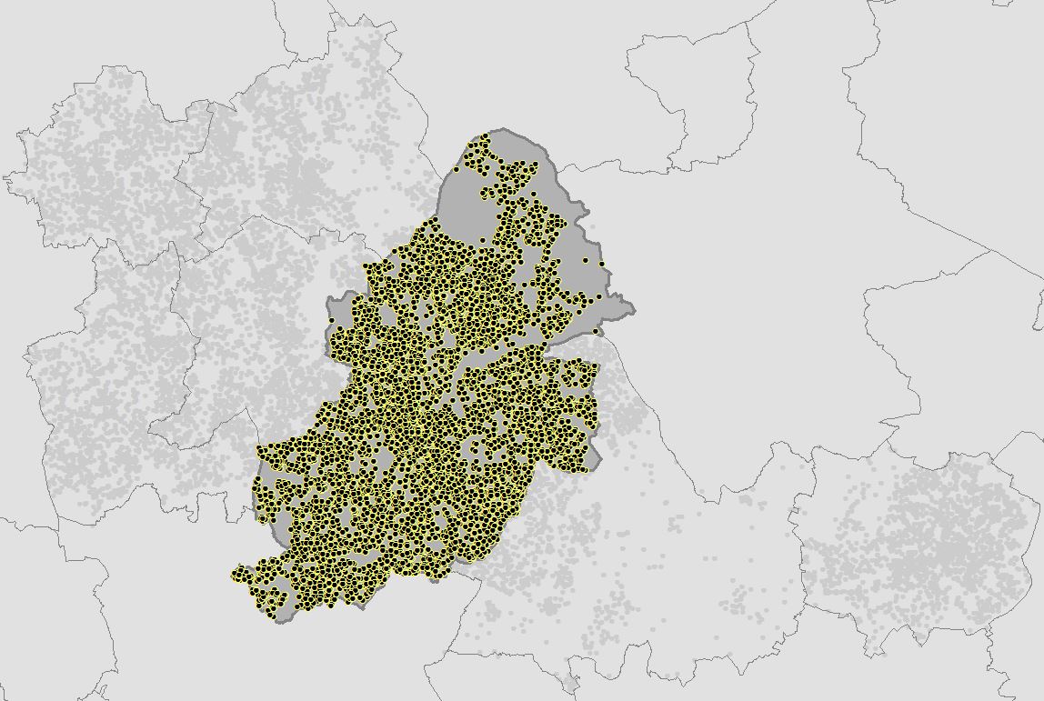
Running the script from The Code section above calculates the Standard Distance for burglaries in Birmingham for 2016 and creates a polygon feature class in the File GDB.

OSGP Mean Center:     407926.695396, 286615.428507
ArcGIS Mean Center:    407926.695396, 286615.428507

OSGP Standard Distance:      6416.076596
ArcGIS Standard Distance:    6416.076596

Also See…

Mean Center
Central Feature
Median Center
Initial Data Assessment

The Resources:

ESRI Guide to GIS Volume 2: Chapter 2 (I highly recommend this book)
see book review here.

Geoprocessing with Python

Python GDAL/OGR Cookbook

Setting up GDAL/OGR with FileGDB Driver for Python on Windows

< The Other Scripts >

1. Extract Burglary Data for West Midlands

import csv, os
from osgeo import ogr, osr

## set the driver for the data
driver = ogr.GetDriverByName("FileGDB")

## path to the FileGDB
gdb = r"C:\Users\Glen B\Documents\my_geodata.gdb"

## ope the GDB in write mode (1)
ds = driver.Open(gdb, 1)

## the coordinates in the csv files are lat/long
source = osr.SpatialReference()
source.ImportFromEPSG(4326)

## we need the data in British National Grid
target = osr.SpatialReference()
target.ImportFromEPSG(27700)

transform = osr.CoordinateTransformation(source, target)

## set the output fc name
output_fc = "WM_Burglaries_2016"

## if the output fc already exists delete it
if output_fc in [ds.GetLayerByIndex(lyr_name).GetName() for lyr_name in range(ds.GetLayerCount())]:
    ds.DeleteLayer(output_fc)
    print "Deleting: {0}".format(output_fc)

out_lyr = ds.CreateLayer(output_fc, target, ogr.wkbPoint)

## define and create new fields
mnth_fld = ogr.FieldDefn("Month", ogr.OFTString)
rep_by_fld = ogr.FieldDefn("Reported_by", ogr.OFTString)
fls_wthn_fld = ogr.FieldDefn("Falls_within", ogr.OFTString)
loc_fld = ogr.FieldDefn("Location", ogr.OFTString)
lsoa_c_fld = ogr.FieldDefn("LSOA_code", ogr.OFTString)
lsoa_n_fld = ogr.FieldDefn("LSOA_name", ogr.OFTString)
crime_fld = ogr.FieldDefn("Crime_type", ogr.OFTString)
outcome_fld = ogr.FieldDefn("Last_outcome", ogr.OFTString)

out_lyr.CreateField(mnth_fld)
out_lyr.CreateField(rep_by_fld)
out_lyr.CreateField(fls_wthn_fld)
out_lyr.CreateField(loc_fld)
out_lyr.CreateField(lsoa_c_fld)
out_lyr.CreateField(lsoa_n_fld)
out_lyr.CreateField(crime_fld)
out_lyr.CreateField(outcome_fld)

## where the downloaded csv files reside
root_folder = r"C:\Users\Glen B\Documents\Crime"

## for each csv
for root,dirs,files in os.walk(root_folder):
    for filename in files:
        if filename.endswith(".csv"):
            csv_path = "{0}\\{1}".format(root, filename)
            with open(csv_path, "rb") as csvfile:
                reader = csv.reader(csvfile, delimiter=",")
                next(reader,None)
                ## create a point with attributes for each burglary
                for row in reader:
                    if row[9] == "Burglary":
                        pnt = ogr.Geometry(ogr.wkbPoint)
                        pnt.AddPoint(float(row[4]), float(row[5]))
                        pnt.Transform(transform)
                        feat_dfn = out_lyr.GetLayerDefn()
                        feat = ogr.Feature(feat_dfn)
                        feat.SetGeometry(pnt)
                        feat.SetField("Month", row[1])
                        feat.SetField("Reported_by", row[2])
                        feat.SetField("Falls_within", row[3])
                        feat.SetField("Location", row[6])
                        feat.SetField("LSOA_code", row[7])
                        feat.SetField("LSOA_name", row[8])
                        feat.SetField("Crime_type", row[9])
                        feat.SetField("Last_outcome", row[10])
                        out_lyr.CreateFeature(feat)

del ds, feat, out_lyr

2. Birmingham Burglaries Only

from osgeo import ogr

## required drivers
shp_driver = ogr.GetDriverByName("ESRI Shapefile")
gdb_driver = ogr.GetDriverByName("FileGDB")

## input boundary shapefile and file gdb
shapefile = r"C:\Users\Glen B\Documents\Crime\Data\GB\district_borough_unitary_region.shp"
gdb = r"C:\Users\Glen B\Documents\my_geodata.gdb"

## open the shapefile in read mode and gdb in write mode
shp_ds = shp_driver.Open(shapefile, 0)
gdb_ds = gdb_driver.Open(gdb, 1)

## reference the necessary layers
shp_layer = shp_ds.GetLayer(0)
gdb_layer = gdb_ds.GetLayerByName("WM_Burglaries_2016")

## filter the shapefile
shp_layer.SetAttributeFilter("NAME = 'Birmingham District (B)'")

## set the name for the output feature class
output_fc = "Birmingham_Burglaries_2016"

## if the output already exists then delete it
if output_fc in [gdb_ds.GetLayerByIndex(lyr_name).GetName() for lyr_name in range(gdb_ds.GetLayerCount())]:
    gdb_ds.DeleteLayer(output_fc)
    print "Deleting: {0}".format(output_fc)

## create an output layer
out_lyr = gdb_ds.CreateLayer(output_fc, shp_layer.GetSpatialRef(), ogr.wkbPoint)

## copy the schema from the West Midlands burglaries
## and use it for the Birmingham burglaries
lyr_def = gdb_layer.GetLayerDefn()
for i in range(lyr_def.GetFieldCount()):
    out_lyr.CreateField (lyr_def.GetFieldDefn(i))

## only get burglaries that intersect the Birmingham region
for shp_feat in shp_layer:
    print shp_feat.GetField("NAME")
    birm_geom = shp_feat.GetGeometryRef()
    for gdb_feat in gdb_layer:
        burglary_geom = gdb_feat.GetGeometryRef()
        if burglary_geom.Intersects(birm_geom):
            feat_dfn = out_lyr.GetLayerDefn()
            feat = ogr.Feature(feat_dfn)
            feat.SetGeometry(burglary_geom)

            ## populate the attribute table
            for i in range(lyr_def.GetFieldCount()):
                feat.SetField(lyr_def.GetFieldDefn(i).GetNameRef(), gdb_feat.GetField(i))
            ## create the feature
            out_lyr.CreateFeature(feat)
            feat.Destroy()

del shp_ds, shp_layer, gdb_ds, gdb_layer

The Usual 🙂

As always please feel free to comment to help make the code more efficient, highlight errors, or let me know if this was of any use to you.