Use the below link to get a hefty discount on my course ArcPy for Data Management and Geoprocessing with ArcGIS Pro at Final Draft Mapping
https://learn.finaldraftmapping.com/cart/?add-to-cart=31491&quantity=1&fdm_apply=GBBLOG90

Use the below link to get a hefty discount on my course ArcPy for Data Management and Geoprocessing with ArcGIS Pro at Final Draft Mapping
https://learn.finaldraftmapping.com/cart/?add-to-cart=31491&quantity=1&fdm_apply=GBBLOG90
Here’s a little function for exporting an attribute table from ArcGIS to a CSV file. The function takes two arguments, these are a file-path to the input feature class or table and a file-path for the output CSV file (see example down further).
First import the necessary modules.
import arcpy, csv
Inside the function we use ArcPy to get a list of the field names.
def tableToCSV(input_tbl, csv_filepath):
    fld_list = arcpy.ListFields(input_tbl)
    fld_names = [fld.name for fld in fld_list]
We then open a CSV file to write the data to.
    with open(csv_filepath, 'wb') as csv_file:
        writer = csv.writer(csv_file)
The first row of the output CSV file contains the header which is the list of field names.
writer.writerow(fld_names)
We then use the ArcPy SearchCursor to access the attributes in the table for each row and write each row to the output CSV file.
        with arcpy.da.SearchCursor(input_tbl, fld_names) as cursor:
            for row in cursor:
                writer.writerow(row)
And close the CSV file.
csv_file.close()
Full script example…
import arcpy, csv

def tableToCSV(input_tbl, csv_filepath):
    fld_list = arcpy.ListFields(input_tbl)
    fld_names = [fld.name for fld in fld_list]
    with open(csv_filepath, 'wb') as csv_file:
        writer = csv.writer(csv_file)
        writer.writerow(fld_names)
        with arcpy.da.SearchCursor(input_tbl, fld_names) as cursor:
            for row in cursor:
                writer.writerow(row)
        print csv_filepath + " CREATED"
    csv_file.close()

fc = r"C:\Users\******\Documents\ArcGIS\Default.gdb\my_fc"
out_csv = r"C:\Users\******\Documents\output_file.csv"

tableToCSV(fc, out_csv)
Feel free to ask questions, comment, or help build upon this example.
Interested in learning ArcPy? check out this course.
I have been using arcpy intermittently over the past year and a half mainly for automating and chaining batch processing to save myself countless hours of repetition. This week, however, I had to implement a facet of arcpy that I had not yet had the opportunity to utilise – the data access module.

The Scenario
A file geodatabase with 75 feature classes each containing hundreds to thousands of features. These feature classes were the product of a CAD (Bentley Microstation) to GIS conversions via FME with data coming from 50+ CAD files. As a result of the conversion each feature class could contain features with various attributes from one or multiple CAD files but each feature class consisted of the same schema which was helpful.

The main issue was that the version number for a chunk of the CAD files had not been corrected. Two things needed to be fixed: i) the ‘REV_NUM’ attribute for all feature classes needed to be ‘Ver2’, there would be a mix of ‘Ver1’ and ‘Ver2’, and ii) in the ‘MODEL_SUMMARY’ if ‘Ver1’ was found anywhere in the text it needed to be replaced with ‘Ver2’. There was one other issue and this stemmed from creating new features and not attributing them, this would have left a ‘NULL’ value in the ‘MODEL’ field (and the other fields). All features had to have standardised attributes. The script would not fix these but merely highlight the feature classes.
OK so a quick recap…
1. Set the ‘REV_NUM’ for every feature to ‘Ver2’
2. Find and replace ‘Ver1’ with ‘Ver2’ in the text string of ‘MODEL_SUMMARY’ for all features.
3. Find all feature classes that have ‘NULL’ in the ‘MODEL’ field.
The Script
Let’s take a look at the thirteen lines of code required to complete the mission.
import arcpy

arcpy.env.workspace = r"C:\Users\*****\Documents\CleanedUp\Feature_Classes.gdb"
fc_list = arcpy.ListFeatureClasses()
fields = ["MODEL", "MODEL_SUMMARY", "REV_NUM"]

for fc in fc_list:
 with arcpy.da.UpdateCursor(fc, fields) as cursor:
  for row in cursor:
   if row[0] == None or row[0] == "":
    print fc + ": Null value found for MODEL"
    break
   if row[1] != None:
    row[1] = row[1].replace("Ver1", "Ver2")
   row[2] = "Ver2"
   cursor.updateRow(row)
The Breakdown
Import the arcpy library (you need ArcGIS installed and a valid license to use)
import arcpy
Set the workspace path to the relevant file geodatabase
arcpy.env.workspace = r"C:\Users\*****\Documents\CleanedUp\Feature_Classes.gdb"
Create a list of all the feature classes within the file geodatabase.
fc_list = arcpy.ListFeatureClasses()
We know the names of the fields we wish to access so we add these to a list.
fields = ["MODEL", "MODEL_SUMMARY", "REV_NUM"]
For each feature class in the geodatabase we want to access the attributes of each feature for the relevant fields.
for fc in fc_list:
 with arcpy.da.UpdateCursor(fc, fields) as cursor:
  for row in cursor:
If the ‘MODEL’ attribute has a None (NULL) or empty string value then print the feature class name to the screen. Once one is found we can break out and move onto the next feature class.
   if row[0] == None or row[0] == "":
    print fc + ": Null value found for MODEL"
    break
We know have a list of feature classes that we can fix the attributes manually.
Next we find any instance of ‘Ver1’ in ‘MODEL_SUMMARY’ text strings and replace it with ‘Ver2’….
   if row[1] != None:
    row[1] = row[1].replace("Ver1", "Ver2")
…and update all ‘REV_NUM’ attributes to ‘Ver2’ regardless of what is already attributed. This is like using the Field Calculator to update.
row[2] = "Ver2"
Perform and commit the above updates for each feature.
cursor.updateRow(row)
Very handy to update the data you need and this script can certainly be extended to handle more complex operations using the arcpy.da.UpdateCursor module.
Check out the documentation for arcpy.da.UpdateCursor
Title: Learning ArcGIS Geodatabases
Author: Hussein Nasser
Publisher: Packt Publishing
Year: 2014
Aimed at: ArcGIS – beginner to advanced
Purchased from: www.packtpub.com

After using MapInfo for four years my familiarity with ArcGIS severely declined. The last time I utilised ArcGIS in employment shapefiles were predominantly used but I knew geodatabases were the way forward. If they were going to play a big part in future employment it made sense to get more intimate with them and learn their inner secrets. This compact eBook seemed like a good place to start…
The first chapter is short and sweet and delivered at a beginner’s level with nice point to point walkthroughs and screenshots to make sure you are following correctly. You are briefed on how to design, author, and edit a geodatabase. The design process involves designing the schema and specifying the field names, data types, and the geometry types for the feature class you wish to create. This logical design is then implemented as a physical schema within the file geodatabase. Finally, we add data to the geodatabase through the use of editing tools in ArcGIS and assign attribute data for each feature created. Very simple stuff so far that provides a foundation for getting set-up for the rest of the book.
The second chapter is a lot bulkier and builds upon the first. The initial task in Chapter 2 is to add new attributes to the feature classes followed by altering field properties to suit requirements. You are introduced to domains, designed to help you reduce errors while creating features and preserve data integrity, and subtypes. We are shown how to create a relationship class so we can link one feature in a spatial dataset to multiple records in a non-spatial table stored in the geodatabase as an object table. The next venture in this chapter takes a quick look at converting labels to an annotation class before ending with importing other datasets such as shapefiles, CAD files, and coverage classes and integrating them into the geodatabase as a single point of spatial reference for a project.
Chapter 3 looks at improving the rough and ready design of the geodatabase through entity-relationship modelling, which is a logical diagram of the geodatabase that shows relationships in the data. It is used to reduce the cost of future maintenance. Most of the steps from the first two chapters are revisited as we are taken through creating a geodatabase based on the new entity relationship model. The new model reduces the number of feature classes and improves efficiency through domains, subtypes and relationship classes. Besides a new train of thought on modelling a geodatabase for simplicity the only new technical feature presented in the chapter is enabling attachments in the feature class. It is important to test the design of the geodatabases through ArcGIS, testing includes adding a feature, making use of the domains and subtypes, and test the attachment capabilities to make sure that your set-up works as it should.
Chapter 4 begins with the premise of optimizing geodatabases through tuning tools. Three key optimizing features are discussed; indexing, compressing, and compacting. The simplicity of the first three chapters dwindles and we enter a more intermediate realm. For indexing, how to enable attribute indexing and spatial indexing in ArcGIS is discussed along with using indexes effectively. Many of you may have heard about database indexing before, but the concept of compression and compacting in a database may be foreign. These concepts are explored and their effective implementation explained.
The first part of the fifth chapter steps away from the GUI of ArcGIS for Desktop and ArcCatalog and switches to Python programming for geodatabase tasks. Although laden with simplicity, if you have absolutely no experience with programming or knowledge of the general concepts well then this chapter may be beyond your comprehension, but I would suggest performing the walkthroughs as it might give you an appetite for future programming endeavours. We are shown how to programmatically create a file geodatabase, add fields, delete fields, and make a copy of a feature class to another feature class. All this is achieved through Python using the arcpy module. Although aimed at highlighting the integration of programming with geodatabase creation and maintenance the author also highlights how programming and automation improves efficiency.
The second part of the chapter provides an alternative to using programming for geoprocessing automation in the form of the Model Builder. The walkthrough shows us how to use the Model Builder to build a simple model to create a file geodatabase and add a feature class to it.
The final chapter steps up a level from file geodatabases to enterprise geodatabases.
“An enterprise geodatabase is a geodatabase that is built and configured on top of a powerful relational database management system. These geodatabases are designed for multiple users operating simultaneously over a network.”
The author walks us through installing Microsoft SQL Server Express and lists some of the benefits of employing an enterprise geodatabase system. Once the installation is complete the next step is to connect to the database from a local and remote machine. Once connections are established and tested an enterprise geodatabase can be created to and its functionality utilised. You can also migrate a file geodatabase to and enterprise geodatabase. The last part of Chapter 6 shows how privileges can be used to grant users access to data that you have created or deny them access. Security is an integral part of database management.
Overall Verdict: for such a compact eBook (158 pages) it packs a decent amount of information that provides good value for money, and it also introduces other learning ventures that come part and parcel with databases in general and therefore geodatabases. Many of the sections could be expanded based on their material but the pagination would then increase into many hundreds (and more) and beyond the scope of this book. The author, Hussein Nasser, does a great job with limiting the focus to the workings of geodatabases and not veering off on any unnecessary tangents. I would recommend using complimentary material to bolster your knowledge with regards to many of the aspects such as entity-relationship diagrams, indexing (both spatial and non-spatial), Python programming, the Model Builder, enterprise geodatabases and anything else you found interesting that was only briefly touched on. Overall the text is a foundation for easing your way into geodatabase life, especially if shapefiles are still the centre of you GIS data universe.
Interested in learning ArcPy? check out this course.
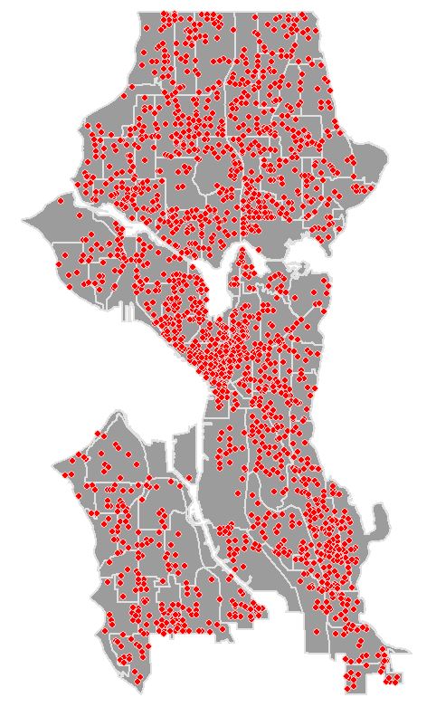
Make sure to read the What is Hotspot Analysis? post before proceeding with this tutorial. This tutorial will serve as an introduction to hotspot analysis with ArcGIS Desktop. You will find links at the bottom of the post that will provide information for further research.
It is often difficult to find real data for use with tutorials so first of all a hat tip to Eric Pimpler, the author of ArcGIS Blueprints, for pointing me towards accessing crime data for Seattle. To follow this tutorial you will need the neighborhoods of Seattle Shapefile which you can download from here and burglary data for 2015 which I have provided a link to here. Use the Project tool from Data Management Tools > Projections and Transformations to project the data into a Projected Coordinate System. For this tutorial I have used UTM Zone 10N. Open, view and if you want style the data in ArcMap.
The presence of spatial clustering in the data is a requisite for hotspot analysis. Moran’s I is a measure of spatial autocorrelation that returns a value ranging from -1 to 1. Perfect dispersion at -1, complete random arrangement at 0, and a north/south divide at +1 indicating perfect correlation.

For statistical hypothesis testing, Moran’s I value can be transformed to a z-zcore in which values greater than 1.96 or smaller than -1.96 indicate spatial autocorrelation that is significant at the 5% level.
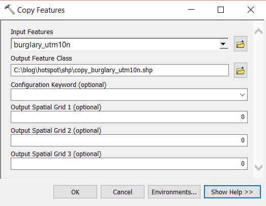
We first need to prepare the data. At the moment each point represent one incident, we need to aggregate the data in some way so that each feature has an attribute with a value in a range. Open the Copy Features tool from Data Management Tools > Features. Create a copy of the burglary point layer. Run the tool and add the new layer to the map.
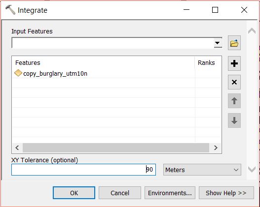
Open the Integrate tool from Data Managemant Tools > Feature Class. Select the copy of the burglary layer as the Input Features and set an XY Tolerance of 90 or 100 meters. Run the tool. This will relocate points within 90m (or 100m) or whatever you set in XY Tolerance field, of each other and stack them on top of one another.
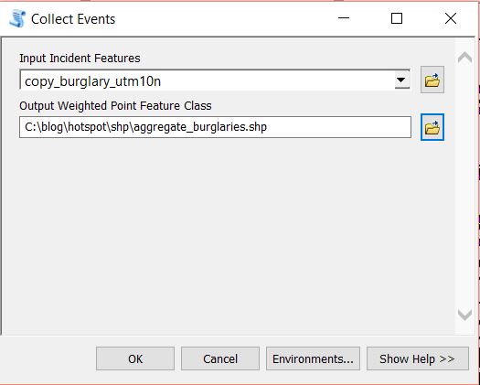
At this moment each point sits on top of another. We need to merge coincident points and make a count of how many were merged at each point. Open the Collect Events tool from Spatial Statistics Tools > Utilities. Set the copy of the burglary layer as the Input Incident Features and set a filepath and name for the Output Weighted Point Feature Class. Run the tool.
The data will be added to the map with graduated symbols, however, we are interested in running further analysis using Moran’s I. If you open the attribute table for the layer you will see a field has been added called ICOUNT. This field holds the count of cooincident points from the Intergrate layer. Open the Spatial Autocorrelation (Moran’s I) from Spatial Statistics Tools > Analyzing Patterns. Set the aggregated burglary layer as the Input Feature Class and ICOUNT as the Input Field. I have left the default setting for the other parameters (see below).
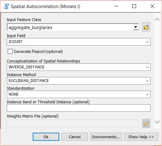
Run the tool by clicking on OK. A summary will display with statistical findings.
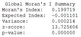
We return a value close to 0.2 and a high z-score. This indicates that clustering exists within the data for high positive values. We are now confident that clustering exists within the dataset and can continue with performing the hotspot analysis.
Remove all layers from map the except the two original layers with the burglary data and the neighborhoods. From the Toolbox navigate to Spatial Statistics Tools > Mapping Clusters and open the Optimized Hotspot Analysis tool. This tool allows for quick hotspot analysis using minimal input parameters and sets/calculates default parameters for those you have no control over. For more control over the statistical elements you can use the Hotspot Analysis (Getis-Ord GI*) tool. For now we will use the optimized approach.
Set the burglary points as the Input Features, name your Output Features (here I have named them ohsa_burg_plygns), select COUNT_INCIDENTS_WITHIN_AGGREGATION_POLYGONS for the Incident Data Aggregation Method and choose the neighborhoods features for the Polygons For Aggregating Incidents Into Counts.

Click OK to run the tool. The ohsa_burg_plygns layer will automatically be added as a layer to the map, if not, add it and turn off all other layers. So what has happened here? The tool has aggregated the point data into the neighborhood polygons. If you open the attribute table for the newly created layer you will see a field names Count_Join which is a count of burglaries per neighborhood. A z-score and a p-score is calculated which enables the detection of hot and cold spots in the data. Remember, a high z-score and a low p-value for a feature indicates a significant hotspot. A low negative z-score and a small p-value indicates a significant cold spot. The higher (or lower) the z-score, the more intense the clustering. A z-score near 0 means no spatial clustering.

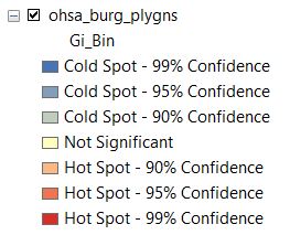
The Gi_Bin field classifies the data into a range from -3 (Cold Spot – 99% Confidence) to 3 (Hot Spot – 99% Confidence), with 0 being non-significant, just take a look at your Table of Contents.
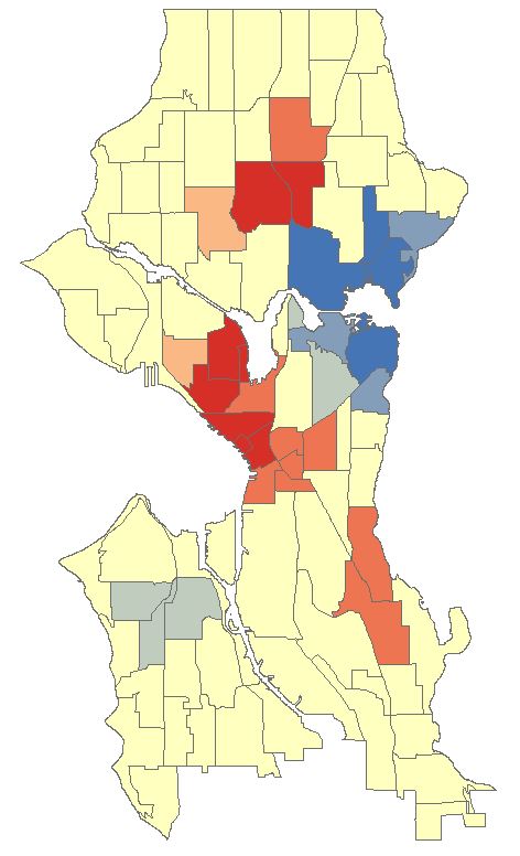
The map should look similar to below. There are several neighborhoods that are statistically significant hotspots. It is important to note that you may need to factor in other data or normalise your data to refine results. Some of the neighborhoods might be densely populated with suburban housing while in others housing may be sparse and bordering towards rural. This may affect findings and you may need to create ratios before analysing. We won’t delve into this here as this tutorial is introductory level (and because I don’t have the data to do so).
Close any attribute tables and turn off all layers in your map. Re-open the Optimized Hotspot Analysis tool and set the input as seen below. This time we will create a fishnet/grid to aggregate the point data to.
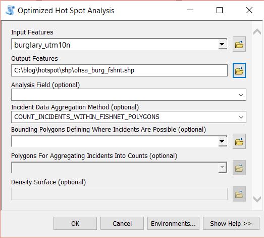
Click OK to run the tool. The tool removes any locational outliers, calculates a cell size, and aggregates the point data to the cells in the grid. Similar to aggregating to polygons the fishnet attribute table will have a join count, z-score, p-score and bin value with the same confidence levels.
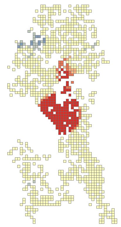 Should attention be entirely focused on the red areas? Copy the fishnet layer and paste it into the data frame. Rename the copy as fishnet_count. Open the properties and navigate to the Symbology tab. Change the Value field to Join_Count, reduce the Classes to 5 and set the classification to Equal Count. Click OK.
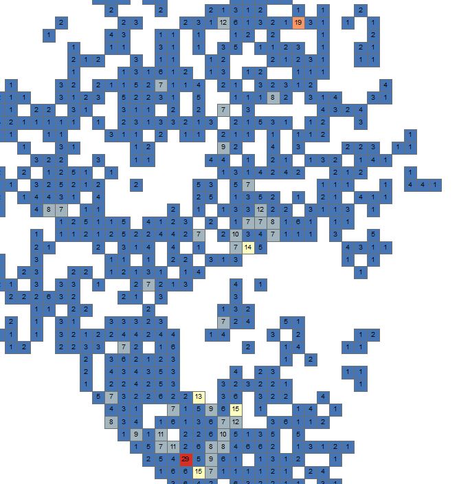
 There will be one red cell and one light red cell in the northern half of the map. Use the zoom tool to zoom-in closer to both features. Turn on the labels for the feature for the Join_Count attribute. Notice that the light-red cell has a count of 19 but in the Hotspot Analysis this was a non-significant area. With the second highest burglary count for a 300m x 300m area surely this area requires some attention. Perhaps all areas outside of significant hotspots with values greater that 15 are a priority? I am not a expert in crime analysis so I’ll leave it up to those sleuth’s.
This just serves to note to make sure that you use all the analysis techniques at your disposal from simple to more advanced, from visual and labels to statistical.
Zoom out to the full extent of the neighborhoods layer and turn off all layers in the map. Re-open the Optimized Hotspot Analysis tool and set the input as seen below. Notice this time we will also create a Density Surface.

Click OK and run the tool. The tool calculates a distance value and converges points that fall within that distance in relation to each other. It then runs the hotspot analysis similar to the previous two examples producing an attribute table with an ICOUNT field, z-score, p-score and bin value for confidence level. The ICOUNT field denotes how many incidents the one point references.

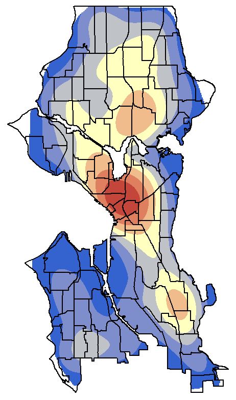
Let’s clip the density raster to the neighborhoods layer. Open the Clip tool from Data Management Tools > Raster > Raster Processing. Set the Input Raster as the density raster, use the neighborhoods layer as the Output Extent, make sure Use Input Features for Clipping Geometry is checked, set and name the Output Raster Dataset.

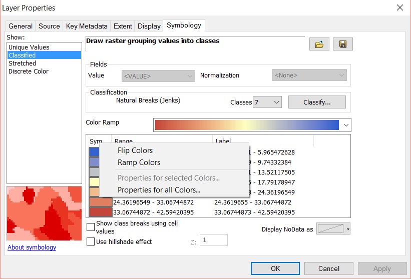
Click OK and run the tool. Add the newly created raster to the map if it hasn’t automatically been added. Make it the only visible layer. Open the properties for the layer and go to the Symbology tab. Select Classified and generate a histogram if asked to. Change the Classes to 7 and the colour ramp to match previous colour schemes. You might need to flip the colour ramp to achieve this.
Open the Display tab and select Bilinear Interpolation from Resample during display dropdown menu. This will smoothen the contour look of the raster. Click OK to view the density surface. Turn on the neighborhoods and make the fill transparent with a black outline.
The Optimized Hotspot Analysis tool is a great place to start but it limits the analysis to default parameters set by the tool or calculated by the tool. For more advanced user control you can use the Hotspot Analysis (Getis-Ord Gi*) tool. You will need to use other tools such as Spatial Join to aggregate your data to polygons and create a Join_Count field, or the Create Fishnet tool to define a grid and then use Spatial Join. Remember to delete any grid cells that have a value of zero prior to running the hotspot analysis.

See the resources below for more information on using Getis-Ord Gi* and what the parameters do especially in relation to the Conceptualization of Spatial Relationships parameter.
ArcGIS Optimized Hotspot Analysis
ArcGIS Mapping Cluster Toolset: Hot Spot Analysis
ArcGIS How Hot Spot Analysis Works
ArcGIS – Selecting a Conceptualization of Spatial Relationships: Best Practices
Crime data was accessed using the ArcGIS REST API and the Socrata Open Data API from the https://data.seattle.gov website. I highly recommend getting your hands on Eric Pimplers ArcGIS Blueprints eBook for a look at exciting workflows with ArcPy and the ArcGIS REST API.
