Labelling in ArcGIS with Formatting Tags and Expressions

Interested in learning ArcPy? check out this course.

I recently sat an interview test where I had to use labelling in ArcGIS Desktop without the aid of the internet or notes for guidance. I must admit I was pretty stumped when it came to formatting labels beyond using the GUI (Labels tab in the Layer Properties) and stepping into the world of expressions, so I decided to rectify this and explore the options. ESRI maintain a fantastic help resource that can be found at here (for 10.2), where you can find what you need to get started. The following examples are some neat ways you can format labels using tags and expressions. They’re quite basic but act as a foundation to build upon.

Open the Layer Properties of the layer you wish to label and switch to the Labels tab. Click on the Expression… button to open the Label Expression window. Switch the Parser at the bottom of the window to Python.

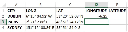
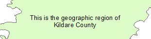
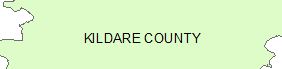
In this first example I will simply concatenate a string with a attribute (also a string), the custom string will be placed on the first line of the label and the attribute of the county name placed on the second. This is achieved with the following…

"This is the geographic region of\n" + [COUNTYNAME]

Labelling - Concatenation
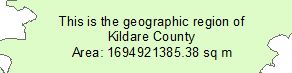
[COUNTYNAME] represents the field names COUNTYNAME in the attribute table of the data I am working with. Next we will concatenate the area on a new line and round the decimal places to two. We cast the area to a string so the concatenation can be preformed.

"This is the geographic region of\n" + [COUNTYNAME] + "\nArea: " + str(round(float([Shape_Area]),2)) + " sq m"

Labelling - Rounding
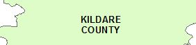
Next we force labels to be presented in upper case text. The Advanced checkbox must be checked to create multiline expressions. You could also replace upper with lower in the below code snippet to force text to be lower case, or replace with title to capitalize the first letter in each word (proper case).

def FindLabel ([COUNTYNAME]):
 label = [COUNTYNAME]
 label = label.upper()
 return label

Labelling - Upper CaseStack text on new lines by using replace. The expression below replaces spaces in the COUNTYNAME attribute with n which forces text after a space onto a new line and removes the space.

def FindLabel ([COUNTYNAME]):
 label = [COUNTYNAME]
 label = label.upper().replace(" ", "\n")
 return label

Labelling - Replace
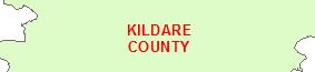
Lets make the text bold  by using format tags. Each tag has an opening < > and closing </ > tag.

def FindLabel ([COUNTYNAME]):
 label = [COUNTYNAME]
 label = label.upper().replace(" ", "\n")
 return "<BOL>" + label + "</BOL>"

Labelling - Bold
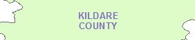
…and then add some colour. Missing RGB values are assumed to be 0.

def FindLabel ([COUNTYNAME]):
 label = [COUNTYNAME]
 label = label.upper().replace(" ", "\n")
 return "<BOL><CLR red='255'>" + label + "</CLR></BOL>"

Labelling - ColourSo how about a custom colour…

def FindLabel ([COUNTYNAME]):
 label = [COUNTYNAME]
 label = label.upper().replace(" ", "\n")
 return "<BOL><CLR red='125' green='105' blue='190'>" + label + "</CLR></BOL>"
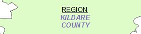
Labelling - Custom Colour…and italics and an underline

def FindLabel ([COUNTYNAME]):
 label = [COUNTYNAME]
 label = label.upper().replace(" ", "\n")
 return "<UND>" + "REGIONn" + "</UND>" + "<BOL><ITA><CLR red='125' green='105' blue='190'>" + label + "</CLR></ITA></BOL>"

Labelling - Italics/Underline
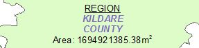
We’ll throw back in the area and format sq m with a superscripted 2 instead…(use SUB if you need to subscript text)

def FindLabel ([COUNTYNAME], [Shape_Area]):
 label = [COUNTYNAME]
 label = label.upper().replace(" ", "\n")
 area = str(round(float([Shape_Area]),2))
 return "<UND>" + "REGIONn" + "</UND>" + "<BOL><ITA><CLR red='125' green='105' blue='190'>" + label + "</CLR></ITA></BOL>" + "nArea: " + area + "m" + "<SUP>" + "2" + "</SUP>"

Labelling - Superscript

Other format tags are <ACP> for all capitals, <SCP> for small capitals, <CHR spacing = ‘200’> for character spacing or <CHR width = ‘150’> for character width, <WRD spacing = ‘200’> for word spacing and <LIN leading = ’25’> for line leading.

Style labels based on attributes. If the area is greater than 1,000,000,000 sq m the label will be styled like the figure above with a colour, if not it will remain black.

def FindLabel ([COUNTYNAME], [Shape_Area]):
 area = str(round(float([Shape_Area]),2))
 label = [COUNTYNAME]
 label = label.upper().replace(" ", "\n")
 if float([Shape_Area]) > 1000000000:
 return "<UND>" + "REGIONn" + "</UND>" + "<BOL><ITA><CLR red='125' green='105' blue='190'>" + label + "</CLR></ITA></BOL>" + "nArea: " + area + "m" + "<SUP>" + "2" + "</SUP>"
 else:
 return "<UND>" + "REGIONn" + "</UND>" + "<BOL><ITA>" + label + "</ITA></BOL>" + "nArea: " + area + "m" + "<SUP>" + "2" + "</SUP>"

Labelling - Attribute StylingThis has just been a quick intro into using expression and format tags for labelling. The Information was found in the online ArcGIS Help that can be found here.

Book Review: Learning QGIS by Anita Graser [eBook]

Title: Learning QGIS (Second Edition)
Author: Anita Graser
Publisher: Packt Publishing
Year: 2014
Aimed at: QGIS – beginner, GIS/Python – knowledgeable
Purchased from: www.packtpub.com

Learning QGISMy New Years resolution is to upgrade skills and software knowledge instead of sitting in front of a TV for hours on end (we’ll see how long this lasts). About six years ago I installed QGIS on my laptop, never used it, removed it, reinstalled it, never used it, removed it and this cycle has continued for each year. I am putting a stop this vicious cycle as of now and aim to become proficient with this well renowned piece of open source software, with my main goal to incorporate Python for automation and develop some plugins. I will become familiar with the software before making the leap to Python.

There’s only so much you can fit into 125 pages and while this book is packed with information on the capabilities of QGIS it certainly leaves you wanting more. I think this is a good problem as it drives you to do your own research and play around with what’s on offer in QGIS based on your own interest.

The book starts off by guiding you through the installation process and then provides a brief description of the interface and available toolbars.

In Chapter 2 we begin to add spatial data (vector and raster) to the map. The link provided to download the sample data didn’t stand the test of time (a year) but was easy to locate with an internet search. We are also introduced to georeferencing, loading data from databases and accessing data from OGC web services, ending without a brief styling tutorial.

The main part of the third chapter walks us through creating and editing geometries and attribute data. We also encounter using the measurements tools, the field calculator, reprojecting and converting files, and joining tabular data.

Chapter 4 presents Spatial Analysis; clipping a raster, terrain analysis, raster calculator, vector to raster and raster to vector conversions, heatmaps, vector geoprocessing (proximity analysis), raster sampling at point locations, density with hexagonal grids, calculate are shares within a region. There is a lot of information in this chapter, without nearly being exhaustive, that emphasizes the analytical capabilities of QGIS.

“Creating Great Maps” is the title of the fifth chapter. Did it hold up to this title? In short, yes, but you are not walked through step by step with someone holding your hand, you are presented with visualization and styling techniques to help you create your own masterpiece. A whole book could be dedicated to this topic.

The final chapter jumps straight into “Extending QGIS with Python” and is certainly not for those just beginning programming with Python. Lines of code are given with a general overview of what’s happening and knowledge of syntax and the API is required here. As a newbie to the QGIS API I found this chapter a bit daunting but time, effort and the will to learn more is a challenge that I accept. The chapter and indeed the book concludes with an example of a processing script and developing and implementing a plugin.

QGIS Python Console

QGIS Python Console

One thing this book has thought me is that QGIS is highly customizable to user preferences and visualizations. My next step is to gain more familiarity with QGIS through available text books and online tutorials before heading down the customization path with Python.

Overall Verdict: Although it was difficult to follow some of the workflows exactly, and this is perhaps because it is more informative than tutorial, I felt this was a good intro to QGIS, what the software has to offer, how to navigate the GUI and the possibilities of extending QGIS with Python. The book cost me a whopping €5.63 from a sale on the Packt Publishing website. This book is packed with info and provided a solid beginning on my quest to QGIS stardom. I am already wondering why it took my so long to break out of that repetitive cycle.

Book Review: Python Scripting for ArcGIS by Paul A. Zandbergen

Title: Python Scripting for ArcGIS
Author: Paul A. Zanbergen
Publisher: ESRI Press
Year: 2013
Aimed at: Python/ArcPy – beginners, ArcGIS – knowledgeable
Purchased from: www.bookdepository.com

Python Scripting for ArcGIS

This book is a fantastic stepping stone for beginners into the enchanted world of ArcPy. ArcPy is a Python site package that provides access to the extensive set of geoprocessing tools available in ArcGIS. Besides enabling programmatic geospatial analysis ArcPy modules also facilitate data management, data conversion and map document management.

I think a quote from the Preface pages of this book aptly sums up what the book is all about.

“a little bit of code goes a long way.”

As an introductory text your eyes will be opened to how small snippets of code can run geoprocessing tools that can form the basis for extensive geospatial analysis. You won’t find in-depth spatial analysis or data management techniques but you will find an easy to read, easy to follow informative text book that provides the theory behind using Python/ArcPy and will act as a reference to the capabilities of ArcPy.

Before purchasing this book I read a number of reviews. While an overwhelming majority applauded the book there where a few who complained about the basic introduction to Python provided. Even though there is a chapter dedicated to creating Python functions and classes one review that sticks out in my mind wanted in-depth object orientated programming for GIS Python which to me is miles beyond the scope of this book. The author does a great job of providing a primer to the Python language but this is not what this book is about. There are a myriad of Python text books for beginners and also online tutorials out there and I would certainly recommend making use of these and getting comfortable with the general syntax, data structures and data types before diving head first into using Python for geospatial activities.

I bought this book because I wanted a foundation for ArcPy that I could build upon. While progressing through the text I was constantly looking to the ArcGIS Resources pages for more information about geoprocessing tools encountered and the syntax required to implement them programmatically. I would recommend using this book in tandem with the Resource pages for the ultimate beginner experience. The book is extremely informative for a beginner’s text but it will be your genuine interest in the material that will take you well beyond what’s on offer here.

The book and topics are well designed with each chapter building upon the previous. The first part introduces the Python language, development environments (PythonWIn and the Interactive Python WIndow in ArcMap), and the basics of geoprocessing. Part two is where you begin your ArcPy experience, writing scripts and learning about ArcPy modules and their capabilities. Part three introduces some specialized tasks such as automating ArcMap workflows through map scripting and error handling is also discussed. Part four provides an introduction to creating your own custom tool.

Some of the more interesting materials I found covered in this book were; working with the mapping module for automating map document tasks, accessing and manipulating data with cursors and the data access module, working with geometries and rasters, and creating custom tools. These will provide the springboard for you to dive into more advanced scripting.

Overall Verdict: The book was a great investment (c. €60). It would be hard to find a better way to introduce yourself to ArcPy. It won’t teach you everything you need to know to build applicable scripts but provides an invaluable foundation. Highly recommended for beginners.

Degrees-Minutes-Second (DMS) to Decimal-Degrees (DD) with Excel

Interested in learning ArcPy? check out this course.

At some point you may be handed data in an Excel file that needs to be imported into a GIS but the coordinate columns are in degrees-minutes-seconds format. For optimum use in the GIS you require the coordinate data in decimal-degrees format. Let’s look at how to achieve this using Excel and the data below for three cities, Dublin, Paris, and Sydney.

Excel Original Data

Add a header for two new columns LONGITUDE and LATITUDE (or calls these whatever suits you, X, Y for example)

Excel Add Columns

Press ALT + F11 to bring up the Microsoft Visual Basic for Applications window. From the Insert dropdown menu, select Module. Copy and paste the code below into the Module window.

Function Convert_Decimal(Degree_Deg As String) As Double
 ' Declare the variables to be double precision floating-point.
 Dim degrees As Double
 Dim minutes As Double
 Dim seconds As Double
 ' Set degree to value before "°" of Argument Passed.
 degrees = Val(Left(Degree_Deg, InStr(1, Degree_Deg, "°") - 1))
 ' Set minutes to the value between the "°" and the "'"
 ' of the text string for the variable Degree_Deg divided by
 ' 60. The Val function converts the text string to a number.
 minutes = Val(Mid(Degree_Deg, InStr(1, Degree_Deg, "°") + 2, _
 InStr(1, Degree_Deg, "'") - InStr(1, Degree_Deg, _
 "°") - 2)) / 60
 ' Set seconds to the number to the right of "'" that is
 ' converted to a value and then divided by 3600.
 seconds = Val(Mid(Degree_Deg, InStr(1, Degree_Deg, "'") + _
 2, Len(Degree_Deg) - InStr(1, Degree_Deg, "'") - 2)) _
 / 3600
 Convert_Decimal = degrees + minutes + seconds
End Function

Close the Microsoft Visual Basic for Applications window and return to the workbook.Click in the first cell under the LONGITUDE header (D2 above) and enter the formula

=IF(RIGHT(B2,1)="W",-Convert_Decimal(B2),Convert_Decimal(B2))

What this is saying is that if the last character of the cell is “W”, for West, then place a negative sign before the entry in the cell. If the last character is not a “W”, leave the entry as positive. See this post for an introduction to Geographic Coordinate Systems. Press enter to populate the cell with the decimal degree value.

Excel Long Function

Highlight the the new cell entry (D2) and grab the bottom right corner and drag down for the other two entries.

Excel Long Function All

Click into the cell under the LATITUDE header (E2) and enter the formula

=IF(RIGHT(C2,1)="S",-Convert_Decimal(C2),Convert_Decimal(C2))

Here, we have replaced the “W” with an “S” for South to account for negative coordinate values. C2 refers to the first cell under the LAT header. Click enter and grab the bottom right corner of the new cell entry and drag down for the other two records.

Excel Lat Function All

The code to convert to decimal degrees was sourced from the Microsoft Support website and can be found here, along with further information about the code and it’s application. The code, itself, does not compensate for negative coordinates so we have added a formula to use with the conversion to compensate for this.

Generate a Projection File (.prj) using Python

This blog has moved to a new home at Final Draft Mapping.

A .prj file contains the coordinate system information for a dataset and is required for ‘on the fly’ projection by GIS software. The file itself is a text file containing information in Well Known Text (WKT) format. The code snippet here shows you how to generate a .prj file, using Python, for your data if the .prj file is missing. See the post on CSV to Shapefile with pyshp for an example of using the function in a workflow. You will need to know what coordinate system the data is in and the EPSG code. For example, to find the EPSG code for WGS84 use a search engine and search for EPSG WGS84. The first site returned is usually http://spatialreference.org/. The EPSG code for WGS84 is 4326.

# function to generate .prj file information using spatialreference.org
def getWKT_PRJ (epsg_code):
     import urllib
     # access projection information
     wkt = urllib.urlopen("http://spatialreference.org/ref/epsg/{0}/prettywkt/".format(epsg_code))
     # remove spaces between charachters
     remove_spaces = wkt.read().replace(" ","")
     # place all the text on one line
     output = remove_spaces.replace("\n", "")
     return output

# create the .prj file
prj = open("filename.prj", "w")
# call the function and supply the epsg code
epsg = getWKT_PRJ("4326")
prj.write(epsg)
prj.close()

The filename should match the name of your data files. For examples, the .prj file for cities.shp or cities.tab should be cities.prj.

If you open the .prj file in a text editor you will see the text below.

GEOGCS["WGS84",DATUM["WGS_1984",SPHEROID["WGS84",6378137,298.257223563,AUTHORITY["EPSG","7030"]],AUTHORITY["EPSG","6326"]],PRIMEM["Greenwich",0,AUTHORITY["EPSG","8901"]],UNIT["degree",0.01745329251994328,AUTHORITY["EPSG","9122"]],AUTHORITY["EPSG","4326"]]

GEOGCS at the beginning of the WKT indicates that EPSG: 4326 is a geographic coordinate reference system (it would be PROJCS if it was a projected coordinate system). The information within the square brackets after DATUM provide the information for the parameters of the datum. We see the name of the datum, ‘WGS_1984’, and the SPHEROID information with a semimajor axis of 6,378,137 m with an inverse-flattening ratio of 298.257223563. The PRIMEM data tells us that it uses Greenwich as the prime meridian (where longitude is zero). UNIT specifies the measurement unit of the coordinate system, here it is ‘degree’, and the 0.0174532925199433 value is required to convert from radians into the stated units.

Open your data in a GIS and make sure that it is displaying correctly in relation to other features.